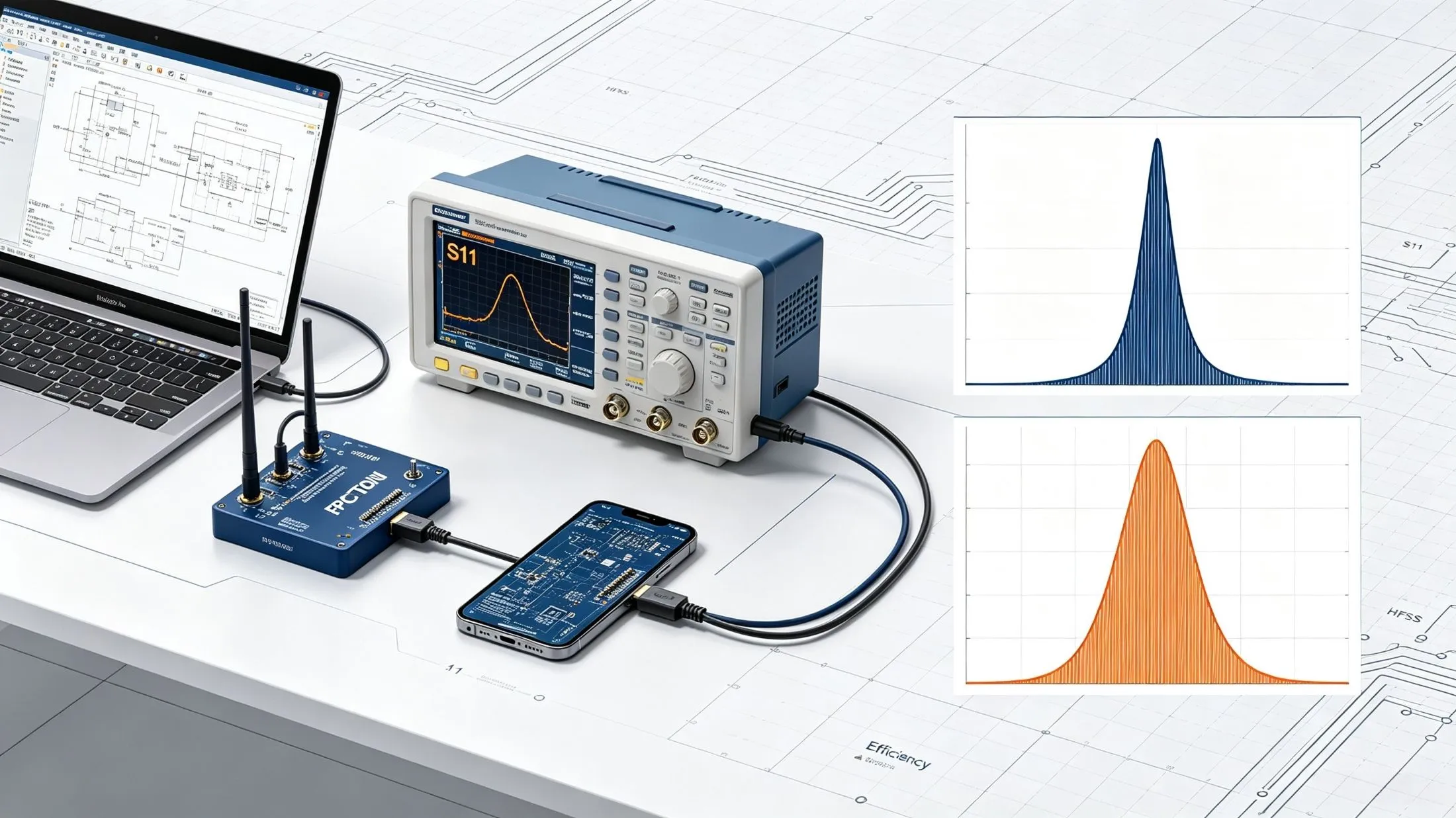
Hardware engineers who debug FPC antennas have almost all encountered the same challenge: the HFSS simulation curves look perfect—with narrow bandwidth and maximum radiation efficiency—but when the board is manufactured, assembled, and tested in the finished device, the results are completely reversed—the S11 bandwidth widens significantly, and the radiation efficiency drops sharply.
This article breaks down the sources of error from a fundamental level, distinguishes between efficiency metrics that are often confused, and provides simulation correction methods that can be implemented immediately, thereby significantly reducing the prototype debugging cycle.
1,Core Underlying Logic
Antenna bandwidth is inversely proportional to the system’s total Q-factor: Simulations, which assume an ideal, low-loss, high-Q single-resonator environment, show narrowband performance and high efficiency; In physical systems, however, the addition of significant losses and parasitic structures causes the total Q-factor to decrease significantly. The resonance peak becomes flatter, and the bandwidth widens; however, continuous energy dissipation leads to a decrease in radiation efficiency.
II,Four Reasons Why Actual Bandwidth Is Actually Wider
Various types of losses reduce the resonant Q-factor (primary cause); simulations default to smooth, ideal copper and pure PI dielectric; In actual products, etching burrs and oxidation on copper foil cause conductor losses, while conductive adhesive, foam, and reinforcement sheets have dielectric loss factors far higher than those of the base material. These losses are equivalent to parallel damping resistors, causing the resonance trough to widen and become shallower.
Simulation of Multi-Resonance Superposition Caused by Parasitic Components: The simulation models only the main body of the antenna, ignoring the distributed capacitance of the pads, component leads, FPC, and metal housing/battery, as well as the parasitic LC of the ground tabs. The superposition of multiple weak resonances is intuitively reflected in a widening of the bandwidth.
When assembling a physical FPC with a smooth impedance curve—accounting for factors such as bending, warping, and uneven gaps between the FPC and the metal ground plane—the equivalent LC values vary more gradually with frequency, naturally broadening the standing wave bandwidth.
The test system incorporates additional damping; the ideal wave port is lossless. Measurements show that metal coupling between the coaxial probe, test socket, and fixture flattens sharp resonance peaks, further broadening the measured bandwidth.
Three,Five Types of Losses That Cause a Sharp Drop in Radiative Efficiency of Physical Objects
Conductor losses: The rough surface of the copper, the skin effect, and current concentration at bends cause significant heat generation from RF energy;
Dielectric loss: The high-frequency loss angle of adhesives, foam, and reinforcing sheets is much greater than that of pure PI;
Eddy current losses in metals: The steel casing and shielding of the battery induce surface currents that absorb radiated energy;
Grounding contact loss: The contact resistance of the spring clip and conductive adhesive increases ohmic loss;
Matching component losses: Physical inductors and capacitors inherently have DC resistance and dielectric loss, which consume transmit power.
Four,Distinguish Between the Two Types of Efficiency to Quickly Pinpoint Faults
Radiation efficiency: Depends solely on the losses in the antenna copper and the dielectric itself; it is unrelated to port reflection;
Total efficiency = radiation efficiency × (1 – reflection coefficient²) Simulation conditions: Reflection at the resonance point is minimal; total efficiency ≈ radiation efficiency; the curve is narrow with a high peak; Physical condition: Losses reduce radiation efficiency; the decrease in Q-factor results in a smoother in-band reflection, producing a wider overall curve with a significantly lower peak.
Five,Practical Implementation Plan for HFSS Simulation Corrections to Reduce the Gap Between Simulation and Physical Results
1.Realistic Material Parameters to Address Inflated Efficiency Figures
Add a surface roughness of 1–3 μm to the copper foil; do not use ideal PEC; use realistic, finite metal conductivity for cells and shielding covers; enter the measured Dk/Df values for the adhesive layer and foam; and add a thin-layer resistance to the ground to simulate contact loss.
2.Complete full-system modeling to simulate parasitic effects
Do not simulate the bare FPC in isolation; model the housing, battery, mainboard ground, matching pads, component leads, and conductive foam to accurately reproduce the parasitic coupling of the entire device.
3.Port and Device Under Real-World Test Conditions
Replace the ideal waveguide port with a coaxial probe model; import the original manufacturer's SP parameter file for the components and discard the ideal LC components; fill the enclosure with realistic plastic instead of using an empty air box.
4.Simple, Equivalent, and Fast Parameter Tuning
When the modeling workload for the entire device is heavy, you can model equivalent stray losses—such as a small resistor in parallel with the antenna port—and the simulation curves will simultaneously exhibit the physical characteristics of “widened bandwidth and reduced efficiency.”
Six,Simple Validation Experiment to Pinpoint the Source of Deviation
Tested the bare FPC antenna on its own: without a housing, foam, or matching components; the response curve closely matches the simulation, with narrow bandwidth and high efficiency;
Retest of the fully assembled unit: After adding the metal casing, conductive adhesive, and foam, an immediate increase in bandwidth and a drop in efficiency were observed. This directly proves that losses and parasitic coupling are the primary sources of discrepancies between simulation and actual performance.
summarize
Simulation = Ideal high Q, low loss, single resonance, characterized by narrow bandwidth and high efficiency; Actual device = Cumulative multi-layer losses + multiple parasitic resonances, resulting in a decrease in total Q-factor and a widening of bandwidth; Various new types of losses continuously consume RF energy, ultimately resulting in measured radiation efficiency that is significantly lower than the simulation results. Optimizing the simulation model before debugging can significantly reduce the cost of repeated PCB revisions for prototypes.